Data Preparation - Part 6 - Moving Average Smoothing

Moving average smoothing is a naive and effective technique in time series forecasting. It can be used for data preparation, feature engineering, and even directly for making predictions. 

After completing this tutorial, you will know:

• How moving average smoothing works and some expectations of your data before you can use it.
• How to use moving average smoothing for data preparation and feature engineering.
• How to use moving average smoothing to make predictions.

A. Moving Average Smoothing

Smoothing is a technique applied to time series to remove the fine-grained variation between time steps. The hope of smoothing is to remove noise and better expose the signal of the underlying causal processes. Moving averages are a simple and common type of smoothing used in time series analysis and time series forecasting. Calculating a moving average involves creating a new series where the values are comprised of the average of raw observations in the original time series.

A moving average requires that you specify a window size called the window width. This defines the number of raw observations used to calculate the moving average value. The moving part in the moving average refers to the fact that the window defined by the window width is slid along the time series to calculate the average values in the new series. There are two main types of moving average that are used: Centered and Trailing Moving Average.

1. Centered Moving Average

The value at time (t) is calculated as the average of raw observations at, before, and after time (t). For example, a center moving average with a window of 3 would be calculated as:

    

        center_ma(t) = mean(obs(t − 1); obs(t); obs(t + 1))

2. Trailing Moving Average

The value at time (t) is calculated as the average of the raw observations at and before the time (t). 

For example, a trailing moving average with a window of 3 would be calculated as:

    

        trail_ma(t) = mean(obs(t − 2); obs(t − 1); obs(t))

B. Daily Female Births Dataset

In this lesson, we will use the Daily Female Births Dataset as an example. This dataset describes the number of daily female births in California in 1959.

C. Moving Average as Data Preparation

Moving average can be used as a data preparation technique to create a smoothed version of the original dataset. Smoothing is useful as a data preparation technique as it can reduce the random variation in the observations and better expose the structure of the underlying causal processes.

The rolling() function on the Series Pandas object will automatically group observations into a window. You can specify the window size, and by default a trailing window is created. Once the window is created, we can take the mean value, and this is our transformed dataset.

New observations in the future can be just as easily transformed by keeping the raw values for the last few observations and updating a new average value. To make this concrete, with a window size of 3, the transformed value at time (t) is calculated as the mean value for the previous 3 observations (t-2, t-1, t), as follows:

            obs(t) = 1/3 × (obs(t − 2) + obs(t − 1) + obs(t))

For the Daily Female Births dataset, the first moving average would be on January 3rd, as follows:

            obs(t) = 1/3 × (obs(t − 2) + obs(t − 1) + obs(t))

                      = 1/3 × (35 + 32 + 30)

                      = 32.333

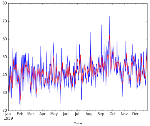
Below is an example of transforming the Daily Female Births dataset into a moving average with a window size of 3 days, chosen arbitrarily.

# moving average smoothing as data preparation

from pandas import read_csv

from matplotlib import pyplot

series = read_csv('daily-total-female-births.csv', header=0, index_col=0, parse_dates=True, squeeze=True)

# tail-rolling average transform

rolling = series.rolling(window=3)

rolling_mean = rolling.mean()

print(rolling_mean.head(10))

# plot original and transformed dataset

series.plot()

rolling_mean.plot(color='red')

pyplot.show()

# zoomed plot original and transformed dataset

series[:100].plot()

rolling_mean[:100].plot(color='red')

pyplot.show()

-----Result-----

Date

1959-01-01 NaN

1959-01-02 NaN

1959-01-03 32.333333

1959-01-04 31.000000

1959-01-05 35.000000

1959-01-06 34.666667

1959-01-07 39.333333

1959-01-08 39.000000

1959-01-09 42.000000

1959-01-10 36.000000

Name: Births, dtype: float64

Line plot of the Daily Female Births dataset (blue) with a moving average (red)

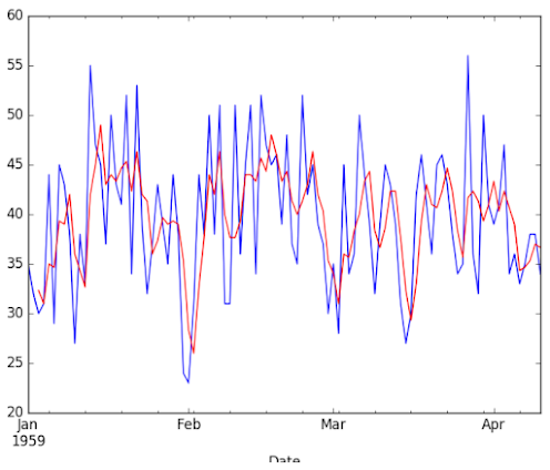
We can zoom in and plot the first 100 observations

Line plot of the first 100 observations from the Daily Female Births dataset (blue)
with a moving average (red)

D. Moving Average as Feature Engineering

The moving average can be used as a source of new information when modeling a time series forecast as a supervised learning problem. In this case, the moving average is calculated and added as a new input feature used to predict the next time step. 

# moving average smoothing as feature engineering

from pandas import read_csv

from pandas import DataFrame

from pandas import concat

series = read_csv('daily-total-female-births.csv', header=0, index_col=0, parse_dates=True, squeeze=True)

df = DataFrame(series.values)

width = 3

lag1 = df.shift(1)

lag3 = df.shift(width - 1)

window = lag3.rolling(window=width)

means = window.mean()

dataframe = concat([means, lag1, df], axis=1)

dataframe.columns = ['mean', 't', 't+1']

print(dataframe.head(10))

-----Result-----

      mean           t        t+1

0    NaN             NaN   35

1    NaN             35.0  32

2    NaN             32.0  30

3    NaN             30.0  31

4    32.333333   31.0  44

5    31.000000   44.0  29

6    35.000000   29.0  45

7    34.666667   45.0  43

8    39.333333   43.0  38

9    39.000000   38.0  27

E. Moving Average as Prediction

The moving average value can also be used directly to make predictions. It is a naive model and assumes that the trend and seasonality components of the time series have already been removed or adjusted for. The moving average model for predictions can easily be used in a

walk-forward manner.

# moving average smoothing as a forecast model

from math import sqrt

from pandas import read_csv

from numpy import mean

from sklearn.metrics import mean_squared_error

from matplotlib import pyplot

series = read_csv('daily-total-female-births.csv', header=0, index_col=0, parse_dates=True,squeeze=True)

# prepare situation

X = series.values

window = 3

history = [X[i] for i in range(window)]

test = [X[i] for i in range(window, len(X))]

predictions = list()

# walk forward over time steps in test

for t in range(len(test)):

length = len(history)

yhat = mean([history[i] for i in range(length-window,length)])

obs = test[t]

predictions.append(yhat)

history.append(obs)

print('predicted=%f, expected=%f' % (yhat, obs))

rmse = sqrt(mean_squared_error(test, predictions))

print('Test RMSE: %.3f' % rmse)

# plot

pyplot.plot(test)

pyplot.plot(predictions, color='red')

pyplot.show()

# zoom plot

pyplot.plot(test[:100])

pyplot.plot(predictions[:100], color='red')

pyplot.show()

-----Result-----

predicted=32.333333, expected=31.000000
predicted=31.000000, expected=44.000000
predicted=35.000000, expected=29.000000
...
predicted=38.666667, expected=37.000000
predicted=38.333333, expected=52.000000
predicted=41.000000, expected=48.000000
predicted=45.666667, expected=55.000000
predicted=51.666667, expected=50.000000
Test RMSE: 7.834

Line plot of the Daily Female Births dataset (blue) with a moving average predictions

Line plot of the first 100 observations from the Daily Female Births dataset (blue)
with a moving average predictions (red)